
UNIT 3: PRODUCER BEHAVIOUR AND SUPPLY
Production: Combining inputs in order to get the output is production.
Production Function: It is the functional relationship between inputs and output in a given state of technology. Q= f(L,K)
Q is the output, L: Labor, K: Capital
Fixed Factor: The factor whose quantity remains fixed with the level of output.
Variable Factor: Those inputs which change with the level of output.
|
Capital |
Labor |
Output |
|
10 |
1 |
50 |
|
10 |
2 |
70 |
|
10 |
3 |
82 |
|
10 |
4 |
92 |
|
10 |
5 |
100 |
Here units of capital used remain the same for all levels of output. Hence it is the fixed factor. Amount of labor increases as output increases. Hence it is a variable factor.
PRODUCTION FUNCTION AND TIME PERIOD
- Production function is a long period production function if all the inputs are varied.
- Production function is a short period production function if few variable factors are combined with few fixed factors.
Time period, can be classified as:
- Very short period or market period
- Short period / short run
- Long period / long run
Market period : is that period where supply / output cannot be altered or changed.
Short period /run : is that period where supply / output can be altered / changed by changing only variable factors of production. In other words fixed factors of production remain fixed.
Long period : is that period where all factors of production are changed to bring about changes in output / supply. No factor is fixed.
Difference between short run & long run :
|
Basis |
Short Run |
Long Run |
|
Meaning |
Only variable factors are changed |
All factors are changed |
|
Price Determination |
Demand is active. |
Both demand & supply play an important role. |
|
Classification |
Factors are classified as fixed & variable. |
All factors are variable. |
Concept of product Refers to volume of goods produced by a firm or an industry during a specific period of time.
Total Product- Total quantity of goods produced by a firm / industry during a given period of time with given number of inputs.
Average product = output per unit of variable input.
APP = TPP / units of variable factor
Average product is also known as average physical product.
Marginal product (MP): refers to addition to the total product, when one more unit of variable factor is employed.
MPn = TPn – TPn-1
MPn = Marginal product of nth unit of variable factor TPn = Total product of n units of variable factor TPn-1= Total product of (n-1) unit of variable factor. n=no. of units of variable factor MP = ATP / An
We derive TP by summing up MP TP = £MP
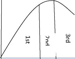
LAW OF VARIABLE PROPORTION OR RETURNS TO A VARIABLE FACTOR
Statement of law of variable proportion: In short period, when only one variable factor is increased, keeping other factors constant, the total product (TP) initially increases at an increasing rate, then increases at a decreasing rate and finally TP decreases.
MPP initially increase then falls but remains positive then 3rd phase becomes negative.
Explanation of law of variable proportion with a schedule and a diagram
Schedule of Law of variable proportion
|
Fixed factor |
Variable factor |
Total product |
Marginal product |
Phase |
|
Land in acres |
Labour |
Units |
Units |
|
|
1 |
0 |
0 |
– |
I – Increasing returns to a factor |
|
1 |
1 |
5 |
5 |
|
|
1 |
2 |
15 |
10 |
|
|
1 |
3 |
30 |
15 |
|
|
1 |
4 |
40 |
10 |
II – diminishing returns to a factor |
|
1 |
5 |
45 |
5 |
|
|
1 |
6 |
45 |
0 |
|
|
1 |
7 |
40 |
-5 |
III – Negative returns to a factor |
Diagram
Y
MPP/TPP
Q-
Q-
X
MPP
X
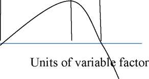
Phase I / Stage I / Increasing returns to a factor.
- TPP increases at an increasing rate
- MPP also increases.
Phase II / Stage II / Diminishing returns to a factor
- TPP increases at decreasing rate
- MPP decreases / falls
- This phase ends when MPP is zero & TPP is maximum
Phase III / Stage III / Negative returns to a factor
- TPP diminishes / decreases
- MPP becomes negative.
Reasons for increasing returns to a factor
- Better utilization of fixed factor
- Increase in efficiency of variable factor.
- Optimum combination of factors Reasons for diminishing returns to a factor
- Indivisibility of factors.
- Imperfect substitutes.
Reasons for negative returns to a factor
- Limitation of fixed factors
- Poor coordination between variable and fixed factor
- Decrease in efficiency of variable factors.
Relation between MPP and TPP
- As long as MPP increases, TPP increases at an increasing rate.
- When MPP decreases, TPP increases diminishing rate.
- When MPP is Zero, TPP is maximum.
- When MPP is negative, TPP starts decreasing.
Short answer questions and Long answer questions
Ans :- Transformation of Input into Output.
Ans :- MP will be zero.
Ans :- Refer time period.
a diagram
6 Marks 6 Marks
4 Marks
- What are the reasons for
- Increasing returns to a factor
- Diminishing returns to a factor
- Negative returns to a factor
- Explain the difference between MPP & TPP.
Giving reasons, state whether the following statements are true or false :
Ans :- False. When there is diminishing returns to a factor, TPP increases at a decreasing rate.
Ans :- False. TPP also increases when MPP decreases but remains positive.
Ans :- False. TPP increases even when there are diminishing returns to a factor.
Ans: – False. Only MPP falls, not TPP. In case of diminishing returns to a factor, TPP increase at diminishing rate.
|
Variable factor unit |
0 |
1 |
2 |
3 |
4 |
5 |
6 |
|
TP (unit) |
0 |
5 |
13 |
23 |
28 |
28 |
24 |
Ans :- MP: 0 5 8 10 5 0 -4
Cost of production : Expenditure incurred on various inputs to produce goods and services. Cost function : Functional relationship between cost and output.
C=f(q)
Where f=functional relationship c= cost of production
q=quantity of product
Money cost : Money expenses incurred by a firm for producing a commodity or service.
Explicit cost : Actual payment made on hired factors of production. For example wages paid to the hired labourers, rent paid for hired accommodation, cost of raw material etc.
Implicit cost : Cost incurred on the self – owned factors of production.
For example, interest on owners capital, rent of own building, salary for the services of entrepreneur etc.
Opportunity cost : is the cost of next best alternative foregone / sacrificed.
Fixed cost : are the cost which are incurred on the fixed factors of production.
These costs remain fixed whatever may be the scale of output. These costs are present even when the output is zero.
These costs are present in short run but disappear in the long run.
Numerical example of fixed cost
|
Output |
0 |
1 |
2 |
3 |
4 |
5 |
|
TFC Rs |
20 |
20 |
20 |
20 |
20 |
20 |
TFC = Total Fixed Cost Diagrammatic presentation of TFC
Y
TFC
to
O
U
X
Output
O
TFC is also called as “overhead cost”, “supplementary cost”, and “unavoidable cost”.
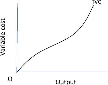
Total Variable Cost : TVC or variable cost – are those costs which vary directly with the variation in the output. These costs are incurred on the variable factors of production.
These costs are also called “prime costs”, “Direct cost” or “avoidable cost”.
These costs are zero when output is zero. Numerical example,
|
Output |
0 |
1 |
2 |
3 |
4 |
5 |
|
TVC |
0 |
10 |
16 |
25 |
38 |
55 |
Diagrammatic presentation of TVC
X
Difference between TVC & TFC
|
Basis |
TVC |
TFC |
|
Meaning |
Vary with the level of output |
Do not vary with the level of output |
|
Time period |
Can be changed in short period |
Remain fixed in short period |
|
Cost at zero output |
Zero |
Can never be zero |
|
Factors of production |
Cost incurred on all variable factors |
Cost incurred on fixed factors of production |
|
Shape of the cost curve |
Upward sloping |
Parallel to x axis |
Total cost : is the total expenditure incurred on the factors and non-factor inputs in the production of goods and services.
It is obtained by summing TFC and TVC at various levels of output.
Relation between TC, TFC and TVC
- TFC is horizontal to x axis.
- TC and TVC are S shaped (they rise initially at a decreasing rate, then at a constant rate & finally at an increasing rate) due to law of variable proportions.
- At zero level of output TC is equal to TFC.
- TC and TVC curves parallel to each other.
TC
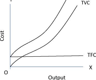
- TC=TFC + TVC
- TFC=TC-TVC
- TVC=TC-TFC
Average cost : are the “cost per unit” of output produced. Average fixed cost is the per unit fixed cost of production. AFC = TFC / Q or output
AFC declines with every increase in output. It’s a rectangular hyperbola. It goes very close to x axis but never touches the x axis as TFC can never be zero.
Average variable cost is the cost per unit of the variable cost of production.
AVC = TVC / output.
AVC falls with every increase in output initially. Once the optimum level of output is reached AVC starts rising.
Average total cost (ATC) or Average cost (AC) : refers to the per unit total cost of production.
ATC = TC / Output AC = AFC + AVC Phases of AC
- phase : When both AFC and AVC fall , AC also fall
- phase : When AFC continue to fall , AVC remaining constant AC falls till it reaches minimum.
- phase : AC rises when rise in AVC is more than fall in AVC.
Important observations of AC , AVC & AFC
- AC curve always lie above AVC (because AC includes AVC & AFC at all levels of output).
- AVC reaches its minimum point at an output level lower than that of AC because when AVC is at its minimum AC is still falling because of fall in AFC.
- As output increases, the gap between AC and AVC curves decreases but they never intersect.
Marginal cost: refers to the addition made to total cost when an additional unit of output is produced.
MCn = TCn-TCn-1 MC = ATC/AQ
Note : MC is not affected by TFC.
Relationship between AC and MC
- Both AC & MC are derived from TC
- Both AC & MC are “U” shaped (Law of variable proportion)
- When AC is falling MC also falls & lies below AC curve.
- When AC is rising MC also rises & lies above AC
- MC cuts AC at its minimum where MC = AC
Important formulae at a glance
- TFC = TC – TVC or TFC=AFC x output or TFC = TC at 0 output.
- TVC = TC – TFC or TVC = AVC x output or TVC =£MC
- TC = TVC + TFC or TC = AC x output or TC = X MC + TFC
- MCn=TCn – TCn-1 or MCn= TVCn – TVCn-1
- AFC = TFC / Output or AFC = AC-AVC or ATC – AVC
- AVC = TVC / Output or AVC = AC-AFC
- AC = TC / Output or AC=AVC + AFC Short answers and Long Answer questions:
- What is cost of production?
- Define cost function.
- What are money costs?
- Distinguish between explicit and implicit costs.
- How do you define an opportunity cost?
- What difference you find between fixed and variable costs?
- Why the fixed cost curve is a horizontal straight line to the X axis?
- Why variable costs are variable?
- What is average cost? How do you derive it?
- Explain AVC, AFC & ATC and explain the relationship between these costs.
- Explain the relationship TC, TFC & TVC.
- With a diagram describe the various phases of AC.
- Bring out the relationship between AC & MC
Ans :- Because TFC can never be zero.
Ans:- AC is the summation of AVC & AFC so AC always lies above AVC & AFC.
Ans:- TVC is zero at zero level of output.
- When TVC is zero at zero level of output, what happens to TFC or Why TFC is not zero at zero level of output?
Ans:- Fixed cost are to be incurred even at zero level of output.
Revenue: – Money received by a firm from the sale of a given output in the market.
Total Revenue: Total sale receipts or receipts from the sale of given output.
TR = Quantity sold x Price (or) output sold x price
Average Revenue: Revenue or Receipt received per unit of output sold.
o AR = TR / Output sold o AR and price are the same. o TR = Quantity sold x price or output sold x price o AR = (output / quantity x price) / Output/ quantity o AR= price
AR and demand curve are the same. Shows the various quantities demanded at various prices.
Marginal Revenue: Additional revenue earned by the seller by selling an additional unit of output.
- MRn = TR n – TR n-1
- MR n = A TR n / A Q
- TR = X MR
Relationship between AR and MR (when price remains constant or perfect competition)
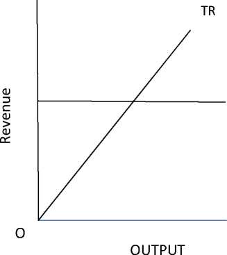
Under perfect competition, the sellers are price takers. Single price prevails in the market. Since all the goods are homogeneous and are sold at the same price AR = MR. As a result AR and MR curve will be horizontal straight line parallel to OX axis. (When price is constant or perfect competition)
Relation between TR and MR (When price remains constant or in perfect competition) When there exists single price, the seller can sell any quantity at that price, the total revenue increases at a constant rate (MR is horizontal to X axis)
|
y |
||
|
Revenue |
AR- IVIR-ri Ice |
|
|
o |
OUTPUT |
x |
Y
AR= MR
X
<D
3
>
O
Y
Price line
Price=AR=MR
X
Quantity
Relationships between AR and MR under monopoly and monopolistic competition
(Price changes or under imperfect competition)
- AR and MR curves will be downward sloping in both the market forms.
- AR lies above MR.
- AR can never be negative.
- AR curve is less elastic in monopoly market form because of no substitutes.
- AR curve is more elastic in monopolistic market because of the presence of substitutes.
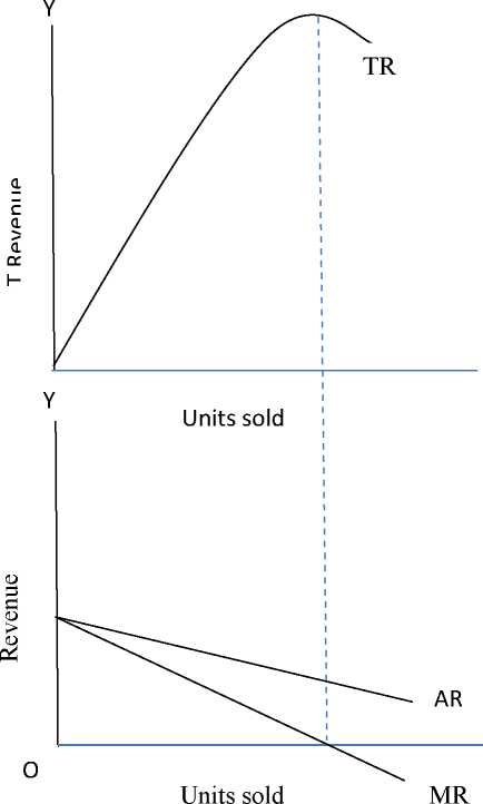
Relationship between TR and MR. (When price falls with the increase in sale of output)
- Under imperfect market AR will be downward sloping – which shows that more units can be sold only at a less price.
- MR falls with every fall in AR / price and lies below AR curve.
- TR increases as long as MR is positive.
- TR falls when MR is negative.
- TR will be maximum when MR is zero.
X
X
Break-even point: It is that point where TR = TC or AR=AC. Firm will be earning normal profit.
Y
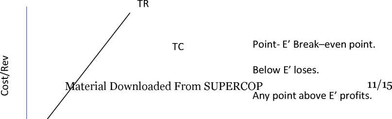
E
Profit
Loss
Shut down p< 0 : A situati O utput firm is able to cover only variable costs or TR = TVC
Formulae at a glance:
- TR = price or AR x Output sold or TR = £ MR
- AR (price) = TR ^ units sold
- MR n = MR n – MR n_i
HOTS
- Can MR be negative or zero.
Ans:- Yes, MR can be zero or negative.
- If all units are sold at same price how will it affect AR and MR?
Ans:- AR and MR will be equal at levels of output.
- What is price line?
Ans:- Price line is the same as AR line and is horizontal to X-axis in perfect competition.
- Can TR be a horizontal Straight line?
Ans:- Yes, when MR is zero.
- What do you mean by revenue?
- Explain the concept of revenue ( TR, AR and MR)
- Define AR
- Prove that AR = price
- Prove that AR is nothing but demand curve.
- Explain the relationships between AR and MR when price is constant and when price falls.
- Explain the relationships between TR and MR when price is constant.
- What is break- even point? Explain with a diagram.
- When the situation of ‘shut – down’ point arises for a firm?
- What happens to TR when a) MR is increasing, b) decreasing but remains positive and c) MR is negative?
Ans:- a) TR increases at an increasing rate.
- TR increases at a diminishing rate.
- TR decreases.
- Why AR is more elastic in monopolistic competition than monopoly?
Ans:- Monopolistic competition market has close substitutes. Monopoly market does not have close substitutes.
Ans:- In perfect competition market the goods are sold at the same price so AR= MR and the TR increases at a constant rate.
Ans:- Yes there can be breakeven point with AR=AC.
- Individual supply refers to quantity of a commodity that an individual firm is willing and able to offer for sale at each possible price during a given period of time.
- Market supply: It refers to quantity of a commodity that all the firms are willing and able to offer for sale at each possible price during a given period of time.
- The supply curve of a firm shows the quantity of commodity (Plotted on the X-axis) that the firm chooses to produce corresponding to two different prices in the market (plotted on the Y-axis)
- Supply Schedule refers to a table which shows various quantity of a commodity that a producer is willing to sell at different prices during a given period of time.
- Determinants of supply are a) state of technology b) input prices c) Government taxation policy.
- Law of supply: It states direct relationship between price and quantity supplied keeping other factors constant.
- Movement along the supply curve: It occurs when quantity supplied changes due to change in its price, keeping other factors constant.
- Shift in supply curve: It occurs when supply changes due to factors other than price.
- Reasons for shift in supply curves: Change in price of other goods, change in price of factors of production, change in state of technology, change in taxation policy.
- Expansion in supply: It occurs when quantity supplied rises due to increase in price keeping other factors constant.
- Contraction of supply: It means fall in the quantity supplied due to fall in price keeping other factors constant.
- Increase in supply refers to rise in the supply of a commodity due to favorable changes in other factors at the same price.
- Decrease in supply: It refers to fall in the supply of a commodity due to unfavorable change in other factors at the same price.
- Price elasticity of supply: The price elasticity of supply of a good measures the responsiveness of quantity supplied to changes in the price of a good.
- Price elasticity of supply = %change in qty supplied/ %change in price.
- Geometric method:
Fig. 1 Fig. 2 Fig.3
Es at a point on the supply curve = Horizontal segment of the supply curve
Quantity supplied
Fig.1: BC/OC>1 fig. 2: BC/OC=1 fig 3. BC/OC<1
FREQUENTLY ASKED QUESTIONS – CBSE BOARD EXAMINATION
One Mark Questions (1M)
- Define the law of supply.
- Define market supply.
- What do you understand by supply curve of a firm?
- What do you mean by elasticity of supply?
- Define supply schedule.
- Define revenue of a firm? OR give meaning of revenue?
- Define Marginal Revenue?
- What is Average revenue?
- When will the marginal revenue become negative?
- What happens to total revenue when Marginal revenue is zero?
- In which market the Average revenue is equal to marginal Revenue?
Three Marks Questions (3M)
- Give reasons for the rightward shift in supply curve?
- Give reasons for the leftward shift in supply curve?
- If the price of the commodity falls by 10 % and consequently the quantity supply decreases by 20 % what will be elasticity of supply?
Four Marks Questions (4 M)
- Briefly explain the geometric method of measuring price elasticity of supply?
- Distinguish between change in supply and change in quantity supplied?
- Explain the movement along the supply curve?
Three OR Four Marks Questions (3M/4M)
1) What changes will take place in marginal Revenue when:
- TR increase at an increasing rate?
- TR increases at a diminishing rate?
2) Complete the following table:
|
Units |
1 |
2 |
3 |
4 |
5 |
6 |
|
Total Revenue |
20 |
56 |
||||
|
Average Revenue |
18 |
|||||
|
Marginal Revenue |
12 |
4 |
0 |
Six Marks Questions (6 M)
- Explain the determinants of supply?
- Explain the relationship between Total Revenue and marginal Revenue using a Schedule and diagram?