Statistics is the Science of collection, organization, presentation, analysis and interpretation of the numerical data.
Useful Terms
1. Limit of the Class
The starting and end values of each class are called Lower and Upper limit.
2. Class Interval
The difference between upper and lower boundary of a class is called class interval or size of the class.
3. Primary and Secondary Data
The data collected by the investigator himself is known as the primary data, while the data collected by a person, other than the investigator is known as the secondary data.
4. Variable or Variate
A characteristics that varies in magnitude from observation to observation. e.g., weight, height, income, age, etc, are variables.
5. Frequency
The number of times an observation occurs in the given data, is called the frequency of the observation.
6. Discrete Frequency Distribution
A frequency distribution is called a discrete frequency distribution, if data are presented in such a way that exact measurements of the units are clearly shown.
7. Continuous Frequency Distribution
A frequency distribution in which data are arranged in classes groups which are not exactly measurable.
Cumulative Frequency Distribution
Suppose the frequencies are grouped frequencies or class frequencies. If however, the frequency of the first class is added to that of the second and this sum is added to that of the third and so on, then the frequencies, so obtained are known as cumulative frequencies (cf).
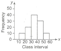
Graphical Representation of Frequency Distributions
(i) Histogram To draw the histogram of a given continuous frequency distribution, we first mark off all the class intervals along X-axis on a suitable scale. On each of these class intervals on the horizontal axis, we erect (vertical) a rectangle whose height is proportional to the frequency of that particular class, so that the area of the rectangle is proportional to the frequency of the class.
If however the classes are of unequal width, then the height of the rectangles will be proportional to the ratio of the frequencies to the width of the classes.
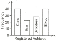
(ii) Bar Diagrams In bar diagrams, only the length of the bars are taken into consideration. To draw a bar diagram, we first mark equal lengths for the different classes on the axis, i.e., X-axis.
On each of these lengths on the horizontal axis, we erect (vertical) a rectangle whose heights is proportional to the frequency of the class.
(iii) Pie Diagrams Pie diagrams are used to represent a relative frequency distribution. A pie diagram consists of a circle divided into as many sectors as there are classes in a frequency distribution.
The area of each sector is proportional to the relative frequency of the class. Now, we make angles at the centre proportional to the relative frequencies.
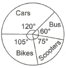
And in order to get the angles of the desired sectors, we divide 360° in the proportion of the various relative frequencies. That is,
Central angle = [Frequency x 360° / Total frequency]
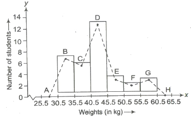
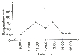
(iv) Frequency Polygon To draw the frequency polygon of an ungrouped frequency distribution, we plot the points with abscissae as the variate values and the ordinate as the corresponding frequencies. These plotted points are joined by straight lines to obtain the frequency polygon.
(v) Cumulative Frequency Curve (Ogive) Ogive is the graphical representation of the cumulative frequency distribution. There are two methods of constructing an Ogive, viz (i) the ‘less than’ method (ii) the ‘more than’ method.
Measures of Central Tendency
Generally, average value of a distribution in the middle part of the distribution, such type of values are known as measures of central tendency.
The following are the five measures of central tendency
1. Arithmetic Mean
2. Geometric Mean
3. Harmonic Mean
4. Median
5. Mode
Arithmetic Mean
The arithmetic mean is the amount secured by dividing the sum of values of the items in a series by the number.
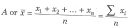
1. Arithmetic Mean for Unclassified Data
If n numbers, x1, x2, x3,….., xn, then their arithmetic mean
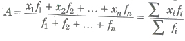
2. Arithmetic Mean for Frequency Distribution
Let f1, f2 , fn be corresponding frequencies of x1, x2,…, xn. Then,
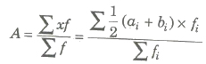
3. Arithmetic Mean for Classified Data
Class mark of the class interval a-b, then x = a + b / 2
For a classified data, we take the class marks x1, x2,…, xn of the classes as variables, then arithmetic mean
Step Deviation Method
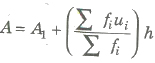
where, A1 = assumed mean
ui = xi – A1 / h
fi = frequency
h = width of interval
4. Combined Mean
If x1, x2,…, xr be r groups of observations, then arithmetic mean of the combined group x is called the combined mean of the observation
A = n1 A1 + n2A2 +….+ nrAr / n1 + n2 +…+ nr
Ar = AM of collection xr
nr = total frequency of the collection xr
5. Weighted Arithmetic Mean
If w be the weight of the variable x, then the weighted AM
Aw = Σ wx / Σ w
Shortcut Method
Aw = Aw‘ + Σ wd / Σ w, Aw‘ = assumed mean
Σ wd = sum of products of the deviations and weight
Properties of Arithmetic Mean
(i) Mean is dependent of change of origin and change of scale.
(ii) Algebraic sum of the deviations of a set of values from their arithmetic mean is zero.
(iii) The sum of the squares of the deviations of a set of values is minimum when taken about mean.
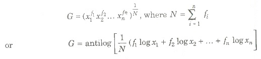
Geometric Mean
If x1, x2,…, xn be n values of the variable, then
G = n√x1, x2,…, xn
or G = antilog [log x1 + log x2 + … + log xn / n]
For Frequency Distribution
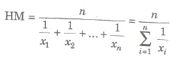
Harmonic Mean (HM)
The harmonic mean of n items x1, x2,…, xn is defined as
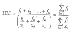
If their corresponding frequencies f1, f2,…, fn respectively, then
Median
The median of a distribution is the value of the middle variable when the variables are arranged in ascending or descending order.
Median (Md) is an average of position of the numbers.
1. Median for Simple Distribution
Firstly, arrange the terms in ascending or descending order and then find the number of terms n.
(a) If n is odd, then (n + 1 / 2)th term is the median.
(b) If n is even, then there are two middle terms namely (n / 2)th and (n / 2 + 1)th terms. Hence,
Median = Mean of (n / 2)th and (n / 2 + 1)th terms.
2. Median for Unclassified Frequency Distribution
(i) First find N / 2, where N = Σ fi.
(ii) Find the cumulative frequency of each value of the variable and take value of the variable which is equal to or just greater than N / 2
(iii) This value of the variable is the median.
3. Median for Classified Data (Median Class)
If in a continuous distribution, the total frequency be N, then the class whose cumulative frequency is either equal to N / 2 or is just greater than N / 2 is called median class.
For a continuous distribution, median
Md = l + ((N / 2 – C) / f) * h
where, l = lower limit of the median class
f = frequency of the median class
N = total frequency = Σ f
C = cumulative frequency of the class just before the median class
h = length of the median class
Quartiles
The median divides the distribution in two equal parts. The distribution can similarly be divided in more equal parts (four, five, six etc.). Quartiles for a continuous distribution is given by
Q1 = l + ((N / 4 – C) / f) * h
Where, N = total frequency
l = lower limit of the first quartile class
f = frequency of the first quartile class
C = the cumulative frequency corresponding to the class just before the first quartile class
h = the length of the first quartile class
Similarly, Q3 = l + ((3N / 4 – C) / f) * h
where symbols have the same meaning as above only taking third quartile in place of first quartile.
Mode
The mode (Mo) of a distribution is the value at the point about which the items tend to be most heavily concentrated. It is generally the value of the variable which appears to occur most frequently in the distribution.
1. Mode for a Raw Data
Mode from the following numbers of a variable 70, 80, 90, 96, 70, 96, 96, 90 is 96 as 96 occurs maximum number of times.
2 For Classified Distribution
The class having the maximum frequency is called the modal class and the middle point of the modal class is called the crude mode.
The class just before the modal class is called pre-modal class and the class after the modal class is called the post-modal class.
Mode for Classified Data (Continuous Distribution)
Mo = l + (f0 – f1 / 2 f0 – f1 – f2) x h
Where, 1 = lower limit of the modal class
f0 = frequency of the modal class
f1 = frequency of the pre-modal class
f2 = frequency of the post-modal class
h = length of the class interval
Relation between Mean, Median and Mode
(i) Mean — Mode = 3 (Mean — Median)
(ii) Mode = 3 Median — 2 Mean
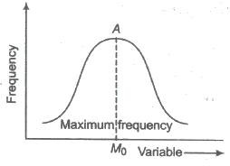
Symmetrical and Skew distribution
A distribution is symmetric, if the same number of frequencies is found to be distributed at the same linear teance on either side of the mode. The frequency curve is bell shaped and A = Md = Mo
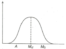
In anti-symmetric or skew distribution, the variation does not have symmetry.
(i) If the frequencies increases sharply at beginning and decreases slowly after modal value, then it is called positive skewness and A > Md > Mo.
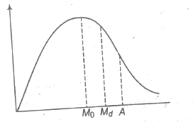
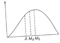
(ii) If the frequencies increases slowly and decreases sharply after modal value, the skewness is said to be negative and A < Md < Mo.
Measure of Dispersion
The degree to which numerical data tend to spread about an average value is called the dispersion of the data. The four measure of dispersion are
1. Range
2. Mean deviation
3. Standard deviation
4. Square Deviation
Range
The difference between the highest and the lowest element of a data called its range.
i.e., Range = Xmax – Xmin
∴ The coefficient of range = Xmax – Xmin / Xmax + Xmin
It is widely used in statistical series relating to quality control in production.
(i) Inter quartile range = Q3 — Q1
(ii) Semi-inter quartile range (Quartile deviation)
∴ Q D = Q3 — Q1 / 2
and coefficient of quartile deviation = Q3 — Q1 / Q3 + Q1
(iii) QD = 2 / 3 SD
Mean Deviation (MD)
The arithmetic mean of the absolute deviations of the values of the variable from a measure of their Average (mean, median, mode) is called Mean Deviation (MD). It is denoted by δ.
(i) For simple (discrete) distribution
δ = Σ |x – z| / n
where, n = number of terms, z = A or Md or Mo
(ii) For unclassified frequency distribution
δ = Σ f |x – z| / Σ f
(iii) For classified distribution
δ = Σ f |x – z| / Σ f
Here, x is for class mark of the interval.
(iv) MD = 4 / 5 SD
(v) Average (Mean or Median or Mode) = Mean deviation from the average / Average
Note The mean deviation is the least when measured from the median.
Coefficient of Mean Deviation
It is the ratio of MD and the mean from which the deviation is measured. Thus, the coefficient of MD
= δ A / A or δ M d / M d or δ M o / M o
Standard Deviation (σ)
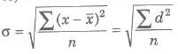
Standard deviation is the square root of the arithmetic mean of the squares of deviations of the terms from their AM and it is denoted by σ.
The square of standard deviation is called the variance and it is denoted by the symbol σ2.
(i) For simple (discrete) distribution
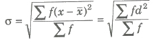
(ii) For frequency distribution
(iii) For classified data
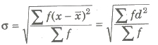
Here, x is class mark of the interval.
Shortcut Method for SD σ =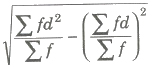
where, d = x — A’ and A’ = assumed mean
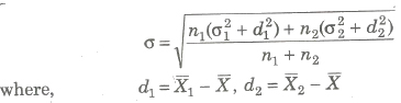
Standard Deviation of the Combined Series
If n1, n2 are the sizes, X1, X2 are the means and σ1, σ2 are the standard deviation of the series, then the standard deviation of the combined series is
Effects of Average and Dispersion on Change of origin and Scale
| Change of origin | Change of scale | |
| Mean | Dependent | Dependent |
| Median | Not dependent | Dependent |
| Mode | Not dependent | Dependent |
| Standard Deviation | Not dependent | Dependent |
| Variance | Not dependent | Dependent |
Important Points to be Remembered
(i) The ratio of SD (σ) and the AM (x) is called the coefficient of standard deviation (σ / x).
(ii) The percentage form of coefficient of SD i.e., (σ / x) * 100 is called coefficient of variation.
(iii) The distribution for which the coefficient of variation is less is called more consistent.
(iv) Standard deviation of first n natural numbers is √n2 – 1 / 12
(v) Standard deviation is independent of change of origin, but it is depend on change of scale.
Root Mean Square Deviation (RMS)
The square root of the AM of squares of the deviations from an assumed mean is called the root mean square deviation. Thus,
(i) For simple (discrete) distribution
S = √Σ (x – A’)2 / n, A’ = assumed mean
(ii) For frequency distribution
S = √Σ f (x – A’)2 / Σ f
if A’ — A (mean), then S = σ
Important Points to be Remembered
(i) The RMS deviation is the least when measured from AM.
(ii) The sum of the squares of the deviation of the values of the variables is the least when measured from AM.
(iii) σ2 + A2 = Σ fx2 / Σ f
(iv) For discrete distribution f =1, thus σ2 + A2 = Σ x2 / n.
(v) The mean deviation about the mean is less than or equal to the SD. i.e., MD ≤ σ
Correlation
The tendency of simultaneous variation between two variables is called correlation or covariance. It denotes the degree of inter-dependence between variables.
1. Perfect Correlation
If the two variables vary in such a manner that their ratio is always constant, then the correlation is said to be perfect.
2. Positive or Direct Correlation
If an increase or decrease in one variable corresponds to an increase or decrease in the other, then the correlation is said to the negative.
3. Negative or Indirect Correlation
If an increase of decrease in one variable corresponds to a decrease or increase in the other, then correlation is said to be negative.
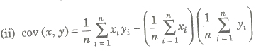
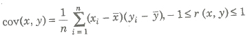
Covariance
Let (xi, yi), i = 1, 2, 3, , n be a bivariate distribution where x1, x2,…, xn are the values of variable x and y1, y2,…, yn those as y, then the cov (x, y) is given by
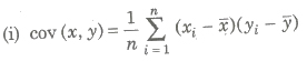
where, x and y are mean of variables x and y.
Karl Pearson’s Coefficient of Correlation
The correlation coefficient r(x, y) between the variable x and y is given
r(x, y) = cov(x, y) / √var (x) var (y) or cov (x, y) / σx σy
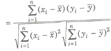
If (xi, yi), i = 1, 2, … , n is the bivariate distribution, then
Properties of Correlation
(i) – 1 ≤ r ≤ 1
(ii) If r = 1, the coefficient of correlation is perfectly positive.
(iii) If r = – 1, the correlation is perfectly negative.
(iv) The coefficient of correlation is independent of the change in origin and scale.
(v) If -1 < r < 1, it indicates the degree of linear relationship between x and y, whereas its sign tells about the direction of relationship.
(vi) If x and y are two independent variables, r = 0
(vii) If r = 0, x and y are said to be uncorrelated. It does not imply that the two variates are independent.
(viii) If x and y are random variables and a, b, c and d are any numbers such that a ≠ 0, c ≠ 0, then
r(ax + b, cy + d) = |ac| / ac r(x, y)
(ix) Rank Correlation (Spearman’s) Let d be the difference between paired ranks and n be the number of items ranked. The coefficient of rank correlation is given by
ρ = 1 – Σd2 / n(n2 – 1)
(a) The rank correlation coefficient lies between – 1 and 1.
(b) If two variables are correlated, then points in the scatter diagram generally cluster around a curve which we call the curve of regression.
(x) Probable Error and Standard Error If r is the correlation coefficient in a sample of n pairs of observations, then it standard error is given by
1 – r2 / √n
And the probable error of correlation coefficient is given by (0.6745) (1 – r2 / √n).
Regression
The term regression means stepping back towards the average.
Lines of Regression
The line of regression is the line which gives the best estimate to the value of one variable for any specific value of the other variable. Therefore, the line of regression is the line of best fit and is obtained by the principle of least squares.
Regression Analysis
(i) Line of regression of y on x,
y — y = r σy / σx (x – x)
(ii) Line of regression of x and y,
x – x = r σx / σy (y — y)
(iii) Regression coefficient of y on x and x on y is denoted by
byx = r σy / σx, byx = cov (x, y) / σ2x and byx = r σx / σy, bxy = cov (x, y) / σ2y
(iv) Angle between two regression lines is given by
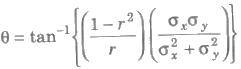
(a) If r = 0, θ = π / 2 , i.e., two regression lines are perpendicular to each other.
(b) If r = 1 or — 1, θ = 0, so the regression lines coincide.
Properties of the Regression Coefficients
(i) Both regression coefficients and r have the same sign.
(ii) Coefficient of correlation is the geometric mean between the regression coefficients.
(iii) 0 < |bxy byx| le; 1, if r ≠ 0
i.e., if |bxy|> 1, then | byx| < 1
(iv) Regression coefficients are independent of the change of origin but not of scale.
(v) If two regression coefficient have different sign, then r = 0.
(vi) Arithmetic mean of the regression coefficients is greater than the correlation coefficient.